A Practical Deformation Monitoring Procedure and Software System for CORS Coordinate Monitoring

Meng Chan LIM and Halim SETAN, Malaysia

¹⁾  This paper illustrates the combination of continuous GPS measurement with robust method for deformation detection to GPS station position change. A window-based software system for GPS deformation detection and analysis via robust method, called Continuous Deformation Analysis System (ConDAS), has been developed at Universiti Teknologi Malaysia. This paper describes the design and architecture of ConDAS and highlights the deformation analysis results from two assessments. The paper is a Malaysian Peer Review paper, which will be presented at FIG Congress 2014 16-21 June, in Kuala Lumpur, Malaysia.

SUMMARY

This paper illustrates the combination of continuous GPS measurement with robust method for deformation detection to GPS station position change. A software system named Continuous Deformation Analysis System (ConDAS) has been developed at Universiti Teknologi Malaysia. It was specially designed to work with high precision GPS processing software (i.e. Bernese 5.0) for coordinate monitoring. The main components of ConDAS are: parameter extraction (from Bernese output), deformation detection (via IWST and S-transformation) and graphical visualisation. Two assessments were included in this paper. Test results show that the system performed satisfactorily, significant displacement can be detected and the stability information of all monitored stations can be obtained. This paper highlights the architecture, the design of the software system and the results.

1. INTRODUCTION

Continuous Global Positioning System (GPS) networks record station position changes with millimetre-level accuracy have revealed that GPS is capable of detecting the significant deformations on various spatial and temporal scales (Ji and Herring 2011; Li and Kuhlmann 2010; Cai et al. 2008; Yu et al. 2006). However, a rigorous deformation analysis technique is still required for preparing a versatile and comprehensive spatial displacement results. To date, several continuous deformation monitoring systems are operational, such as SCIGN (Hudnut et al. 2001), GOCA (Jager et al. 2006) and DDS (Danisch et al. 2008). This study employs a robust method known as Iteratively Weighted Similarity Transformation (IWST) and final S-Transformation to the daily GPS position time series.

A window-based software system for GPS deformation detection and analysis via robust method, called Continuous Deformation Analysis System (ConDAS), has been developed at Universiti Teknologi Malaysia. It is a software system that solely designed to work with high precision GPS processing software (i.e. Bernese 5.0) for coordinate monitoring. The main components of ConDAS are: parameter extraction (from Bernese output), deformation detection and graphical visualisation. All these components are integrated in one environment using MATLAB.

This paper describes the design and architecture of ConDAS and highlights the deformation analysis results from two assessments. In fact, the robust IWST method that employed by ConDAS is typically used for structural deformation monitoring such as dam, slope and etc. However, this study combines IWST and final S-Transformation techniques to Continuous Operating Reference Station (CORS) coordinate monitoring. Larger monitoring area was analysed using robust method for the first time. Promising results have been obtained through the assessment.

2. SYSTEM DEVELOPMENT APPROACH

This study is devoted to develop a software system that adapts to GPS deformation detection and analysis for GPS CORS network. Due to the extraordinary demands for displacement detection accuracy, high precision GPS processing software, namely Bernese 5.0 is employed. Figure 1 outlines the process of entire study.

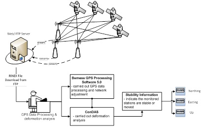
Figure 1: The outline of developed deformation detection system

ConDAS is designed to work with Bernese software for deformation detection and analysis, thus this study comprises of two parts: GPS data processing strategy (via Bernese) and deformation analysis strategy (via ConDAS).

2.1 GPS Data Processing Strategy

There are numbers of GPS deformation monitoring study using Bernese to process GPS data (Haasdyk et al. 2010; Hu et al. 2005; Jia 2005; Janssen 2002; Vermeer 2002). By implementing the Bernese software, data cleaning, cycle slip detection, ambiguity resolution and network adjustment of GPS data all can be achieved to meet the desired criteria. The processing procedure using Bernese Processing Engine (BPE) with double difference is illustrated in Figure 2.

Basically, the entire GPS processing step is divided into three parts: preparation, pre-processing and processing. The preparation part deals with computing a priori coordinate file, preparing the orbit and earth orientation files in Bernese formats, converting RINEX files to Bernese format, synchronising the receiver clocks to GPS time and producing an easy to read overview of available data. Meanwhile, the pre-processing part handles the creation of single difference files, editing of the cycle slips and removal of suspect observation. The processing part is responsible to resolve the ambiguity. After computing a solution with real valued ambiguities the Quasi Ionosphere Free (QIF) strategy is used to resolve ambiguities to their integer numbers. Subsequently, the processing part computes and provides the fixed ambiguity solution. A summary results file is saved and dispensable output files are removed at the final stage of processing.

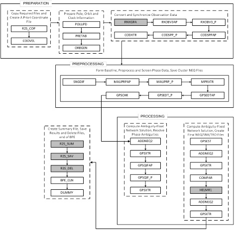
Figure 2: Double difference GPS processing method using BPE

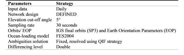
The GPS data are post-processed using Bernese 5.0 software. In order to capitalise the deformation analysis context, some GPS data processing parameters and models were carefully configured as listed in Table 1. In spite of the general script in Bernese GPS software 5.0, some processing scripts are slightly change to well fit the requirement of deformation analysis. For instance, the function of script SNGDIF (in the pre-processing part) is used to generate single-difference files from two zero-difference files. In other word, program SNGDIF is employed to form baselines only from zero-difference observation files. There are plenty of options to be selected for generating the single-difference observation files for network solution. In general the option OBS-MAX guarantees the best performance for the processing of a network using correct correlations. However, there is another option that fit the demand of deformation analysis, called DEFINED option, in which only the predefined baselines from a baseline definition file are created. The selection of DEFINED option has significant impact on the determination of total number of parameters involved for every epoch.

Table 1: Parameters and models used in GPS data processing

Generally, Bernese GPS Software allows user to control the processing strategies or even skip certain redundant scripts (highlighted in Figure 2) during processing. Thus, for deformation analysis purpose, the following redundant scripts are skipped: HELMR1, R2S_SUM, R2S_SAV and R2S_DEL.

Besides, the command line of searching clock correction file (P1C1yymm.DCB and P1P2yymm.DCB) had been removed or disable from the R2S_COP script that stored in the directory C:\GPSUSER\SCRIPT. Eventually, the GPS data processing was performed without the clock correction file and it has been verified that no significant influence on final Bernese output by incessant trial and error. At last, three types of result files were generated for every 24-hour epoch, for instance: a priori coordinate file and adjusted coordinate file in STA folder (e.g.: APR110010.CRD & R1_110010.CRD), along with covariance file in OUT folder (e.g.: R1_11001.COV).

2.2 Deformation Analysis Technique and Software Development

The determination of deformations is mainly formed from two parts. The first is the measurement of deformation and the second is the analysis of these measurements (Aguilera et al. 2007). However, deformation analysis using the geodetic method mainly consists of a two-step analysis via independent adjustment of the network of each epoch, followed by deformation detection between the two epochs (Setan and Singh 2001). In this case, network adjustment is handled by Bernese 5.0 software and ConDAS carries out the two-epoch deformation analysis.

Generally, conventional deformation analysis applied in geodesy (Caspary 1988) extracts the deformation vectors and the variance-covariance matrix. In this classification, Iteratively Weighted Similarity Transformation (IWST) tends to compute the displacement vector and its variance-covariance matrix by iteratively changing weight matrix, W. In fact, IWST method belongs to the family of “robust” methods. IWST method finds the best datum, with minimal distorting influence on the vector of displacement (Chrzanowski et al. 1994). However, for the deformation analysis here we strongly recommended the final S-transformation (with respect to stable reference points) after the IWST is applied. A flow chart of IWST with final S-Transformation method is illustrated in Figure 3. For further computation of IWST and S-Transformation, please refer to Lim (2012), Lim et al. (2010) and Chen et al. (1990).

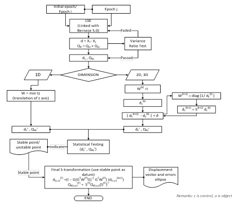
Figure 3: Flow chart of IWST with final S-Transformation that deployed in ConDAS

Two-epoch deformation analysis was employed in this study. From Figure 3, when comparing the two epochs of data (Epoch i: Xi , Qx ; Epoch j: Xj , Qx ) , the vector of displacements (dc) and (Qdc) its cofactor matrix are calculated as shown in Lim et al (2010):

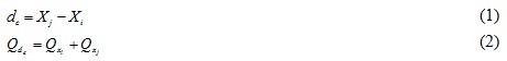
(In Equations (1) and (2), Xi and Xj must be in the same datum. An S-transformation with respect to the same datum must be conducted before the calculation of d (Figure 3).

At the beginning of the deformation analysis, the first matrix which must be computed is the weight matrix, W. For the first iteration (k=1), the matrix W is equal to I (i.e. W=I), where all the diagonal elements are 1 and all other elements are 0. In the second (k+1) and all subsequent iterations, the diagonal elements of the weight matrix are defined as:

For 1-D networks, there are some differences for the calculation of d’ and Qd’. Firstly, the displacements d are arranged in increasing order. The median is assigned unit weight 1 and zero weight is assigned to the other displacements d. If the total number of d is an even number, the two middle (median) displacements d are assigned unit weight 1 and zero weight is assigned to the other displacement d (Chen et al. 1990). Then, the new vector of displacements d’ and its cofactor matrix Qd’ are (Chen et al. 1990):

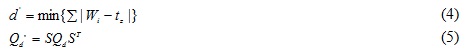
where tz = mean value of the middle displacements and
di = the displacement of point i.
S = similarity transformation matrix =
G = inner constraint matrix

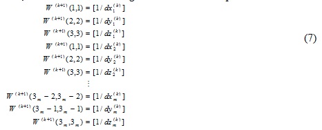
For a 2-D network, the elements of the weight matrix W are computed as follow:

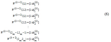
where k is the iteration number.

For a 3-D network, the elements of the weight matrix W are computed as follow:

It is possible that some may approach zero during the iterations, causing numerical instabilities, because becomes very large. There are two ways to solve this problem (Chen et al. 1990):
i. Setting a lower bound (e.g. 0.0001 m). If is smaller than the lower bound value, its weight is set to zero, or
ii. Replacing the weight matrix as , where is a tolerance value.
In this study, the first solution has been chosen and it is preferable to limit the weight matrix for avoiding the long computation.

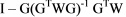
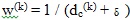
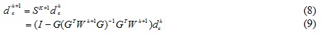
After that, is computed using the following equation (Chen et al. 1990)

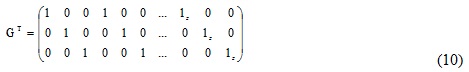
The G matrix is an inner constraint matrix. The dimensions of the G matrix are different for 1-D, 2-D and 3-D networks. For a GPS network, the matrix G is illustrated as Equation 10.

Further details are given in Chen et al. (1990) and Chrzanowski et al. (1994). The iterative procedure continues until the absolute differences between the successive transformed displacements d are smaller than a tolerance value , 0.0001 m (Chen et al. 1990):

In the last iteration, a final S-transformation is performed to get the actual value of the displacement vector by using stable reference points (as verified by the previous IWST analysis) as datum. Consequently, elements of weight matrix, W are assigned 1 for stable reference points and 0 for other points to achieve the final S-transformation. Hence, the principle of congruency testing (Setan and Singh, 2001) is used for calculating the actual deformation displacement vector. In the final iteration, the displacement vector and the final cofactor matrix of displacement vector are computed as:

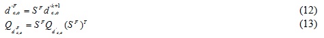
where for stable reference points and 0 for other points based on the previous IWST analysis.

When the vectors of the displacements and the variance-covariance matrix of each point are computed, the stability information of each point can be determined through a single point test. The displacement values and the variance-covariance matrix are compared with a critical value. Assuming the point i is tested, then, the algorithms are as follow (Chen et al. 1990; Setan and Singh 2001)

:
 

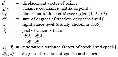
where

If the above test passes then the point is assumed to be stable at a significance level α. Otherwise, if the test fails then the point is assumed to have moved.

In principle, ConDAS has been developed using Matrix Laboratory (MATLAB). This software system is tentatively developed to detect the unstable stations in a deformation monitoring network by IWST method and S-Transformation to analyse the GPS results in the deformation perspective. Figure 4 illustrates the overall workflow of ConDAS.

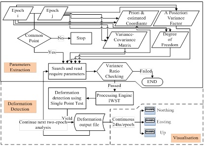
Figure 4: Architecture of ConDAS (Lim et al., 2011)

As an overall, ConDAS consists of three modules: parameters extraction module, deformation detection module and visualisation module. The architecture and function of modules are described respectively as following.

2.2.1 Parameters Extraction Module

After high accuracy coordinates computation from Bernese GPS software, a posteriori variance factor, degree of freedom and variance-covariance matrices can be obtained from the result files. These parameters are required in order to perform the two-epoch deformation analysis. In other words, these parameters are the inputs of deformation analysis. For this study, a Bernese parameter extraction module has been created using MATLAB as illustrated in Figure 5(a). It was designed to suit with Bernese in order to extract the required parameters according to the format of Bernese results files. A warning message will pop out if the specify parameters are unavailable in the Bernese output file. A deformation input file in text file (.txt) was generated after parameters extraction from Bernese output as shown in Figure 5(b).

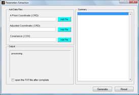
Figure 5(a): GUI of parameters extraction

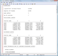
Figure 5(b): Example format of deformation input file.

2.2.2 Deformation Detection Module

The core of deformation analysis program is the implementation of IWST algorithm. However, initial checking of data and test on variance ratio are important to ensure that common points, similar approximate coordinates and same points names are used in two epochs. Thus, there is a statistic test termed variance ratio test that need to be conducted in order to determine the compatible weighting between two epochs, and any further analysis should be stopped at this stage if test is rejected. The test statistic is referred to as Equation 15 (Lim et al. 2010; Setan and Singh 2001).

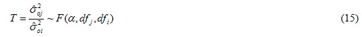
with j and i represent the larger and smaller variance factors, F is the Fisher’s distribution, is the chosen significance level (typically = 0.05) and and are the degrees of freedom for epoch i and j respectively.

In this module, two-epoch deformation analysis were performed in two stages: i) stability analysis of reference stations using IWST and single point test; and ii) deformation analysis of all stations by final S-transformation and single point test. Indication of a set of stable control stations was crucial in order to compute the displacement vectors of all monitored stations respectively. Deformation detection module of ConDAS as illustrated in Figure 6(a) currently utilises a single point test in detecting displacement that reject any point with its displacement extends beyond the confidence region (Chrzanowski et al. 1994). It is flagged as unstable if a given point fails the test at the specified confidence level. At the final stage of program, a summarised deformation output file could be generated as shown in Figure 6(b). It contains the summary of file used, statistical summary and station information whether the station is flagged as moved or stable.

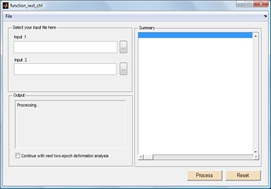
Figure 6(a): GUI of deformation detection module

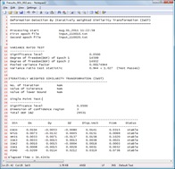
Figure 6(b): Output file of deformation detection module

2.2.3 Visualisation Module

The function of the visualisation module is twofold: i) to view the stability results of every two-epoch analysis; ii) to generate the deformation trend over a selected period. In fact, the stability results in numerical and graphical modes are provided and visualised together with error ellipse and displacement vector for every monitored station. Besides, fluctuation of displacement vector over a period can be visualised via this module. Some data statistics (e.g.: maximum, minimum and standard deviation values over that particular period) also can be obtained from visualisation module. Figure 7 presents the GUI of visualisation module

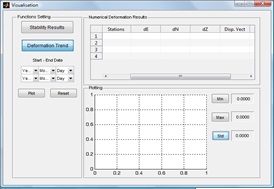
Figure 7: GUI of visualisation module.

3. TEST RESULTS

Two test results were included in this paper for assessment purpose. Due to the CORS coordinate monitoring is the aim of the study, two sets of GPS data were collected from Malaysia Real Time Kinematic GNSS Network (MyRTKnet) and Iskandar Malaysia CORS Network (ISKANDARnet) (Shariff et al. 2009). The first set of data was used to validate the software system by Aceh earthquake incident, the latter one was utilised to monitor the displacement trend of every GPS stations within the network.

3.1 Test Results 1: Validation of System using Aceh Earthquake

Lately, the validation of the entire system was conducted by using the existing GPS data set from MyRTKnet. The processed data set started from 4th Dec 2004 until 31st Dec 2004 (i.e. before and after the Aceh earthquake incident on 26th Dec 2004). Total six of IGS stations (ALIC, DARW, DGAR, HYDE, KARR and KUNM) have been chosen as the control points and two stations from MyRTKnet: JHJY and LGKW were selected as object points. Figure 8 illustrates network distribution of selected IGS and MyRTKnet stations.

 
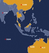
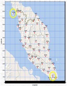
Figure 8: Network distribution of six IGS stations and two MyRTKnet stations

However, only the stable control point (among the selected IGS station) that being verified by ConDAS can be used as datum to compute the displacement vectors of object points. Throughout the analysis, all stations were stable before the earthquake happen. However, the results show the LGKW station was moved start from 26th Dec 2004 and onwards. These results are similar with findings from Jhonny (2010). Figures 9 and 10 illustrate the fluctuation of displacement vectors for JHJY and LGKW.

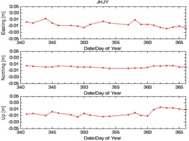
Figure 9: Fluctuation of displacement vectors of station JHJY in Easting, Northing and Up.

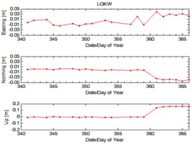
Figure 10: Fluctuation of displacement vectors of station LGKW in Easting, Northing and Up.

From Figure 9, there were no significant movements detected at station JHJY during the incident occurred and the days onwards. The maximum displacement vectors were varied from 0.003m to 0.023m. However, significant movements were detected at station LGKW at the day of year 361 and onwards (Figure 10). The displacement vectors were diverged from 0.007m to 0.167m. Table 2 shows the stability information in numerical results.

Table 2: The displacement vectors of station JHJY and LGKW

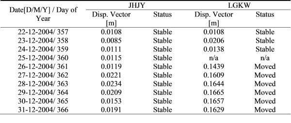
n/a = data not available

3.2 Test Results 2: Deformation Trend of ISKANDARnet

There were seven stations in the deformation monitoring network, four from the IGS stations were used as reference (i.e. COCO, NTUS, PIMO, XMIS) and three stations from ISKANDARnet (ISK1, ISK2 and ISK3) were used as object points as illustrated in Figure 11.

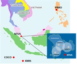
Figure 11: The deformation monitoring network for ISKANDARnet

GPS data processing and two-epoch deformation analysis were performed using two years (1st Jan 2010 – 31st Dec 2011) GPS data. However, ISKANDARnet was undergone some rigorous on-site maintenance during March, July and August of year 2010 and early of April until Jun of year 2011. Thus, no GPS data was available on that specified period. 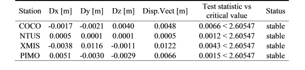After the GPS data processing was carried out with Bernese software, two-epoch deformation analysis (at 5% significance level) were performed in two stages: i) stability analysis of reference stations using IWST; and ii) deformation analysis of all stations. The stability of reference stations was vital in order to select a set of stable reference stations to conduct the analysis for all stations in the monitoring network. The results of stability analysis of two epoch’s data (4th and 5th Jan 2010) in Table 3 confirmed that all four reference stations were stable.

Table 3: Stability analysis of the four reference stations using IWST

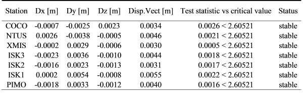
Subsequently, deformation analysis of all seven stations was carried out via final S-transformations based on the stable reference points (Table 3). All seven stations were verified as stable (Table 4). Consequently, the results obtained illustrate that the movement experienced by the GPS CORS stations at cm level can be detected. However, there was no significant movement as shown in Table 4.

Table 4: Stability of all monitoring stations using final S-Transformation based on four stable reference points

Next, GPS data (1st Jan 2010 – 31st Dec 2012) have been processed and analysed continually using the devised technique. The epoch on 4th Jan 2010 and 1st Jan 2011 were selected as reference epoch for year 2010 and year 2011 respectively that any epochs against it. The results of stability analysis show all the stations are stable. The fluctuation of CORS stations: ISK1, ISK2 and ISK3 can be revealed through plotting in Northing, Easting and Up. Figure 12(a), 12(b), 12(c) show the variation of ISK1, ISK2 and ISK3 in Easting, Northing and Up for year 2010. Nevertheless, Figure 13(a), 13(b), 13(c) show the variation of ISK1, ISK2 and ISK3 in Easting, Northing and Up for year 2011.

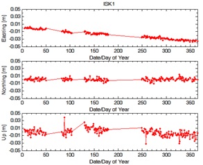
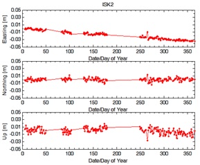
Figure 12(a): Variation of displacement vectors of ISK1 in Easting, Northing and Up for year 2010.	Figure 12(b): Variation of displacement vectors of ISK2 in Easting, Northing and Up for year 2010.
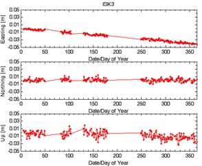
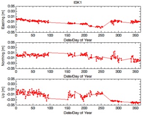
Figure 12(c): Variation of displacement vectors of ISK3 in Easting, Northing and Up for year 2010.	Figure 13(a): Variation of displacement vectors of ISK1 in Easting, Northing and Up for year 2011.
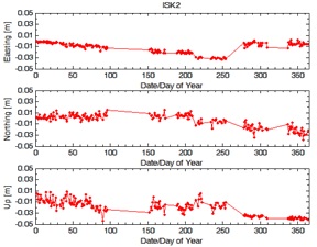
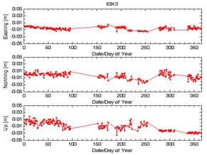
Figure 13(b): Variation of displacement vectors of ISK2 in Easting, Northing and Up for year 2011.	Figure 13(c): Variation of displacement vectors of ISK3 in Easting, Northing and Up for year 2011.

With respect to Figure 12(a), Figure 12(b) and Figure 12(c), Easting component of ISK1, ISK2 and ISK3 were suspicious that undergo some position changes throughout 2010. However, the displacements were considered still under the safe condition and this three monitored stations were deemed to be stable based on the computed deformation analysis results. As an overall, the largest standard deviation of ISK1, ISK2 and ISK3 reached 1.3 centimetres. 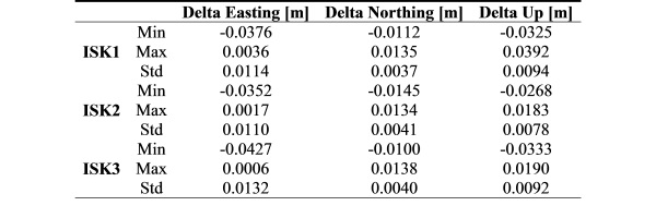It illustrates the obtained results was promising enough in the context of consistency. Table 5 shows the data statistics of ISKANDARnet stations in year 2010.

Table 5: Statistical analysis of ISK1, ISK2 and ISK3 for year 2010

Consequently, regarding to Figure 13(a), Figure 13(b) and Figure 13(c) deformation analysis of ISKANDARnet was interrupted due to some rigorous on-site maintenance and software up-grading throughout the year 2011. GPS data was not available that caused gaps to occur all the way in the plotting. In particular, largest standard deviation of ISK1, ISK2 and ISK3 achieved 1.5 centimetres. From Figure 13(a), Figure 13(b) and Figure 13(c), Up component of three monitored stations was suddenly slumped from day of year 280 until day of year 365. Further site investigation was needed to ensure the location was free from threats. 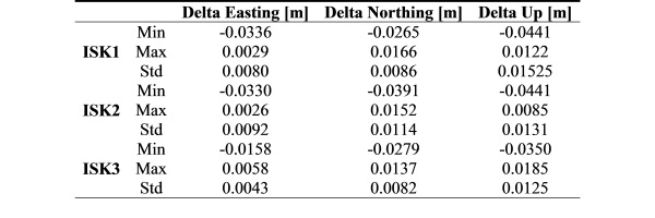Nevertheless, all monitored stations were deemed to be stable and no significant displacement was detected in year 2011. Table 6 illustrates the data statistics of ISK1, ISK2, and ISK3 for year 2011.

Table 6: Statistical analysis of ISK1, ISK2 and ISK3 for year 2011

4. CONCLUSION

In this paper, the skeleton of continuous deformation analysis and visualisation of GPS CORS has been illustrated. A combination of strategy is devised to develop a compatible deformation detection software system for CORS coordinate monitoring. To attain the millimeter accuracy, some special processing strategies had been applied in the Bernese GPS software. Three types of output files from Bernese software were extracted for deformation detection and analysis. Consequently, a windows-based software system for GPS deformation detection via IWST and final S-transformation methods, called ConDAS, has been described. It has been proven to have potential for providing high-quality stability information for CORS network. The test results show the suitability of this software system for practical applications. Furthermore, the obtained results are very promising, indicating the suitability of combining IWST and final S-transformation techniques for CORS coordinate monitoring. The future works tend to improve the flexibility of this software system in terms of data searching, loading and code embedding towards a fully automated deformation monitoring system.

Acknowledgements

The authors would like to thank Department of Survey and Mapping Malaysia (DSMM) for providing valuable MyRTKnet GPS data. The authors are grateful to the following agencies for research funds: Ministry of Science, Technology and Innovation (MOSTI) for Science Fund (Vot. 79350), Ministry of Higher Education (MOHE) for RUG (Vot. Q.J130000.7127.02J69) and Land Surveyors Board (LJT) Malaysia. The authors also grateful to GNSS & Geodynamics Research Group (FKSG, Universiti Teknologi Malaysia) which provide the research facility for data processing purposes.

REFERENCES

Aguilera, D.G., Lahoz, J.G. and Serrano, J.A.S., 2007. First Experiences with The Deformation Analysis of A Large Dam Combining Laser Scanning and High-accuracy Surveying. XXI International CIPA Symposium. 01-06 October. Athens, Greece.

Cai, J., Wang, J., Wu, J., Hu, C., Grafarend, E. and Chen, J., 2008. “Horizontal deformation rate analysis based on multiepoch GPS measurement in Shanghai.” J. Surv. Eng., 134(4), 132-137.

Caspary, W.F., 1988. Concept of Network and Deformation Analysis. Monograph 11, School of Surveying, University of New South Wales, Kensington, 183pp.

Chen, Y.Q., Chrzanowski, A. and Secord, J.M., 1990. A Strategy for the Analysis of the Stability of Reference Points in Deformation Surveys. CISM Journal ACSGC, 44(2): 141-149.

Chrzanowski, A., Caissy, M., Grodecki, J. and Secord, J., 1994. Software Development and Training for Geometrical Deformation Analysis. UNB Final Report. Contract No. 23244-2-4333/01-SQ.

Danisch, L., Chrzanowski, A., Bond, J. and Bazanowski, M., 2008. Fusion of Geodetic and MEMS Sensors for IntegratedMonitoring and Analysis of Deformation. Proceedings of the 4th IAG Symposium on Geodesy for Geotechnical and Structural Engineering & 13th International (FIG) Symposium on Deformation Measurement and Analysis. 12–15 May, Lisbon, Portugal.

Haasdyk, J., Roberts, C. and Janssen, V., 2010. Automated Monitoring of CORSnet-NSW using the Bernese Software. FIG Congress 2010, Sydney, Australia, April 11-16.

Hu, Y.J., Zhang, K.F. and Liu, G.J., 2005. Deformation Monitoring and Analysis using Regional GPS Permanent Tracking Station Networks. FIG Working Week. Cairo, Egypt, April 16-21.

Hudnut, K. W., Bock, Y., Galetzka, J. E.,Webb, F. H. and Young, W. H., 2001. The Southern California Integrated GPS Network (SCIGN). Proceedings of the 10th FIG International Symposium on Deformation Measurements. Orange, CA, USA, 19–22 March: 129–148.

Jager, R., Kalber, S. and Oswald, M., 2006. GNSS/GPS/LPS based Online Control and Alarm System (GOCA) – Mathematical Models and Technical Realisation of a System for Natural and
Geotechnical Deformation Monitoring and Analysis. Proceedings of the 3rd IAG Symposium on Geodesy for Geotechnical and structural Engineering and 12th FIG Symposium on Deformation
Measurements. 22–24 May, Baden, Austria.

Janssen, V., 2002. GPS Volcano Deformation Monitoring. GPS Solutions. 6: 128-130, DOI 10.1007/s 10291-002-0020-8.

Jhonny, 2010. Post-Seismic Earthquake Deformation Monitoring in Peninsular Malaysia using Global Positioning System. M. Sc. Thesis, pp. 58. Universiti Teknologi Malaysia.

Ji, K.H., and Herring, T.A., 2011. Transient Signal Detection using GPS Measurements: Transient Inflation at Akutan Volcano, Alaska, During Early 2008, Geophys. Res. Lett., 38, L06307, doi:10.1029/2011GL046904.

Jia, M.B., 2005. Crustal Deformation from the Sumatra-Andaman Earthquake. AUSGEO news, issue 80.

Li, L. and Kuhlmann, H., 2010. “Deformation detection in the GPS real-time series by the multiple kalman filters model”. J. Surv. Eng., 136(4), 157-164.

Lim, M.C., Halim Setan and Rusli Othman, 2010. A Strategy for Continuous Deformation Analysis using IWST and S-Transformation. World Engineering Congress 2010, Kuching, Sarawak, Malaysia, 2-5 August.

Lim, M.C., Halim Setan and Rusli Othman, 2011. Continuous Deformation Monitoring Using GPS And Robust Method: ISKANDARnet. Joint International Symposium on Deformation Monitoring, Hong Kong, China, 2-4 November.

Lim, M.C., 2012. Deformation monitoring procedure and software system using robust method and similarity transformation for ISKANDARnet. M.Sc. thesis. Universiti Teknologi Malaysia.

Setan, H. and Singh, R., 2001. Deformation Analysis of a Geodetic Monitoring Network. Geomatica. 55(3), 333-346.

Shariff, N.S.M., Musa, T.A., Ses, S., Omar, K., Rizos, C. and Lim, S., 2009. ISKANDARnet: A Network-Based Real-Time Kinematic Positioning System in ISKANDAR Malaysia for Research Platform. 10th South East Asian Survey Congress (SEASC), Bali, Indonesia, August 4-7.

Vermeer, M., 2002. Review of The GPS Deformation Monitoring Studies Commissioned by Posiva Oy on the Olkiluoto, Kivetty and Romuvaara sites, 1994-2000. STUK-YTO-TR 186. Helsinki.

Yu, M., Guo, H. and Zou, C.W., 2006. Application of Wavelet Analysis to GPS Deformation Monitoring. IEEE Xplore. 0-7803-9454-2/06, 670-676.

BIOGRAPHICAL NOTES

Lim Meng Chan was a M.Sc. student at the Dept of Geomatic Engineering, Faculty of Geoinformation and Real Estate, Universiti Teknologi Malaysia (UTM). She holds B. Eng. (Hons) in Geomatic (2008) and M.Sc. in Satellite Surveying (2013). Her master project focuses in the area of GPS for continuous deformation monitoring under supervision of Prof. Dr. Halim Setan and Mr. Rusli Othman.

Dr. Halim Setan is a professor at the Faculty of Geoinformation and Real Estate, Universiti Teknologi Malaysia. He holds B.Sc. (Hons.) in Surveying and Mapping Sciences from North East London Polytechnic (England), M.Sc. in Geodetic Science from Ohio State University (USA) and Ph.D from City University, London (England). His current research interests focus on precise 3D measurement, deformation monitoring, least squares estimation, laser scanning and 3D modelling.

CONTACTS

Prof. Dr. Halim Setan
Department of Geomatic Engineering,
Faculty of Geoinformation and Real Estate
Universiti Teknologi Malaysia (UTM)
81310 Johor Bharu
Johor
MALAYSIA
Tel. +607-5530908
Fax + 607-5566163
Email: halim@utm.my
Web site: -