GRAV-D: Using Aerogravity to Produce a Refined Vertical Datum

Daniel ROMAN & Xiaopeng LI,  United States

¹⁾  This paper focuses upon the aerogravity science necessary to support the production of a cm-level accurate geoid height model. The background is the Gravity for the Redefinition of the American Vertical Datum (GRAV-D) Project in 2008 with a goal of developing a new vertical datum realized through a regional (continental scale) geoid height model.  The paper was presented at the 2014 FIG Congress in Kuala Lumpur, Malaysia. 

SUMMARY

The U.S. National Geodetic Survey instituted the Gravity for the Redefinition of the American Vertical Datum (GRAV-D) Project in 2008 . This geoid model will serve as the realization of a new vertical height system in the U.S.A., replacing NAVD 88. Collaboration with Canada, Mexico and other countries in North America, Central America and the Caribbean will ensure that this model can serve as a regional vertical datum, which can be readily linked to a future World Height System. In order to produce such a model, significant (3-8 mGal) biases that exist in many of the 1400 different terrestrial gravity surveys over the U.S.A. must be detected and mitigated. Furthermore, 10-100 km wide near-shore gaps in oceanic gravity surveys needed to be surveyed. Satellite models do not have sufficient resolution to do either of these tasks. Hence, aerogravity profiles were collected to enhance the satellite gravity field model for such uses. However, in order to use the aerogravity data, trackwise biases needed to be first corrected. A simplified approach was taken to determine and remove biases in the aerogravity profiles using a reference model determined by blending EGM2008 with GOCO03S. A comparison between aerogravity and the modified reference model off the Coast of the Northeastern U.S. highlighted areas of systematic difference at the +/- 3 mGal level with lateral extents of about 100 km. These features would translate into an equivalent 5-10 cm of systematic error in a geoid model and indicate possible errors in the surface gravity data used in EGM2008. A similar analysis over the Great Lakes region demonstrated +/- 10 mGal biases with the NGS surface gravity data and clearly marked which surface gravity profiles need to be addressed. More sophisticated techniques will be developed for this process in the future. The intent though is that aerogravity will be used to detect and mitigate the NGS surface survey data, which largely lack metadata that might otherwise eliminate these errors. In this manner then, the satellite, airborne, and terrestrial data will made consistent so as to produce seamless gravity field model for accurate and precise vertical control.

1. INTRODUCTION
1.1 Background

The National Geodetic Survey (NGS) is responsible for maintaining access to the National Spatial Reference System (NSRS) within the United States. The two principal aspects of the NSRS of importance to surveyors are the North American Datum of 1983 (NAD 83) and the North American Vertical Datum of 1988 (NAVD 88). It has been well established by previous studies (Snay and Soler 2000, Smith et al. 2013a) that both of these official datums have significant (meter level) systematic inaccuracies. Although both datums demonstrate considerable internal consistency, significant problems with absolute accuracy require that these datums be replaced. This is particularly true for NAVD 88 where 30-50 cm regional features are detected and the difference between the zero elevation surface of the datum and the best satellite-based estimates of the geoid is over a meter in the Pacific Northwest. Both will be replaced in 2022 by new geometric and geophysical datums as is outlined in the NGS Ten-Year Strategic Plan (NGS 2013). This paper will focus upon the aerogravity science necessary to support the replacement of NAVD 88 with a new vertical datum realized through a regional (continental scale) geoid height model.

Such models are regularly developed from global models that are refined with regional surface gravity data. Essentially, the local gravity field enhances the global model to produce a regional model of suitable quality. Any systematic errors in the surface gravity data will be removed first to achieve the desired cm-level of accuracy as given in the NGS Ten-Year Plan.

After 2022, the vertical datum will be realized by a combination of GNSS measurement and a geoid height model. Once horizontal coordinates are determined through GNSS technology, the geoid height at that location will be interpolated from the gridded geoid height model, and a simple linear formula will be applied to derive the orthometric height. Since the expectation is that the GNSS-derived geometric coordinates will be cm-level accurate, then the geoid height model must be of a similar accuracy.

1.2 Paper Organization

This paper is focused on the use of aerogravity data to search for systematic errors in the surface gravity data and to evaluate their potential impact if not removed. Aerogravity profiles are available from the NGS website for the Gravity for the Redefinition of the American Vertical Datum (GRAV-D) Project (http://www.ngs.noaa.gov/GRAV-D/). These data were minimally filtered so as to maximize recovery of the gravity signal amplitude. Small biases with respect to satellite gravity fields (generally < 2 mGal) and other noise remain and are left to the discretion of the user to remove depending on their requirements. For geoid modeling, it is helpful to remove these biases from the aerogravity data to produce a more coherent recovery of the gravity field. Such a consistent field better reveals geophysical signals expressed across multiple profiles. The aerogravity data, overflying all, can quality check the surface gravity field, comprised of data sourced from terrestrial gravity measurements, shipborne surveys, and gravity determined from satellite altimeters, and can serve to unify them into a seamless whole.

The next subsection provides more background on the GRAV-D Project. Section 2 focuses on the aerogravity that has been collected as a part of GRAV-D. It presents brief subsections on how missions were planned and processed. Section 3 analyzes data over the Northeast U.S. to demonstrate the removal of biases from the aerogravity profiles, and how that aids in determining defects in the existing reference field models. The aerogravity signal is also downward continued to the surface for a direct comparison to the existing point surface gravity data held by NGS. This last step is most useful for two reasons. Firstly, the downward continued airborne data can be used in place of the surface gravity data for geoid modeling, at least for selected spectral bands where the airborne data is superior (Smith et al., 2013b). Secondly, it identifies potential biases in surface gravity surveys which must be corrected for the resulting geoid model to meet the desired cm-level accuracy. It is this second use which is discussed later in the paper. The last section provides for an outlook and details some of the future work required to meet the 2022 deadline.

1.3 Why GRAV-D?

The Gravity-Lidar Study of 2006 (GLS06) (Roman 2007) collected aerogravity over the northern Gulf of Mexico over Alabama and Mississippi. Gravity grids were generated from the aerogravity and surface gravity data held in the NGS gravity database. A prominent disagreement with 3-5 mGal features existed between the airborne and surface gravity data in the region (about 150 km x 250 km) west of Mobile Bay. Three East-West and twelve North-South aerogravity profiles crossing the region all contained signal that differed systematically from what was seen in the terrestrial data. A 2008 surface gravity survey (Roman et al. 2010) over the same region confirmed this difference, and definitively put the source of the discrepancy on the historic terrestrial gravity data. Terrestrial data were collected at 10 km intervals using LaCoste-Romberg relative meters tied to multiple absolute gravity sites determined from a Micro-g LaCoste-Romberg FG-5 absolute gravimeter. The new surface gravity data agreed with the aerogravity, and both showed the same systematic difference with the gravity data from the NGS database. The effect of this 3-5 mGal systematic difference produced 10 cm of inaccuracy in the geoid model for that region. With the requirement for a cm-level accurate geoid model, the existing gravity measurements in the database are insufficient, at least for this region. This problem in the surface data would not have been identified without the airborne data.

Saleh et al. (2013) demonstrated that significant (3-8 mGals) biases exist in hundreds of the 1400 different terrestrial surveys that comprise the two million gravity points across the U.S.A. These biases would make it impossible to derive a cm-level accurate geoid model; thus the data must be "cleaned" somehow to remove these biases.

The intent of this project is to use the aerogravity to bridge the spectral gap between satellite and surface gravity data. Spherical Harmonic Models (SHM’s) are used to represent the global gravity field. Satellite data dominate the longest wavelengths (λ) at lower degree harmonics in the SHM’s, which is where most of the power is located. In Figure 1, the blue line shows the power by degree harmonic. The variance (power) is higher to the left and falls off to the right. The lower harmonics to the left correlate to larger features and longer wavelengths, which means that satellite data are more sensitive to larger features in the gravity field.

The length of the aerogravity surveys (generally 500 km long profiles) ensures that they contain signal at wavelengths that are also observed by various satellite gravity missions, such as GRACE (Drinkwater et al. 2007) and GOCE (Pail et al. 2011). Since the aerogravity data are measured from a moving platform at higher altitude (details below), it does not contain as much of the short wavelength signal. The shortest wavelength signal, which extends farthest to the right in Figure 1, is where larger degree harmonics correlate to smaller scale features with less power. The red boxes in Figure 1 highlight the portions of the power spectra where the aerogravity overlaps with both the satellite observed gravity field and surface gravity data.

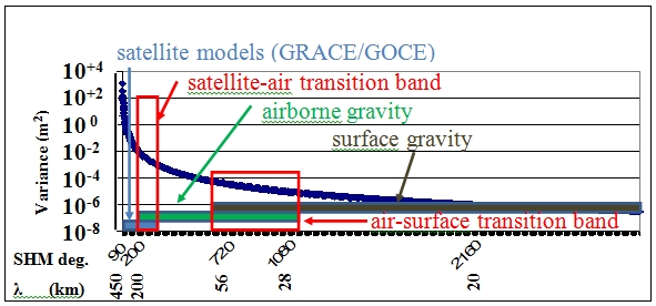
Figure 1 Power Spectrum plot of gravity field (blue line). Most power is at longest wavelengths (λ) at left on the lowest degree harmonics, where satellite (light blue bar) data dominate. Surface data (brown bar) contain the shortest to the right. Aerogravity (green bar) overlaps both parts of spectrum (red boxes).

The satellite model will serve to unify regional models by providing long wavelength consistency. Any inconsistencies in the long wavelengths of the aerogravity will be ignored in favor of the signal from satellite data. Ideally, the satellite model is augmented by the aerogravity to produce a combined reference model independent of surface gravity data in order to evaluate the surface gravity data. The surface data will then be normalized by removal of biases and long to intermediate signal trends. All data would then be consistent and could be joined into a seamless gravity field model useful for defining a vertical reference system that is both accurate and as precisely repeatable as currently leveling methods. Hence, the GRAV-D Project becomes a necessary component for replacing NAVD 88 in 2022.

2. GRAV-D AEROGRAVITY SURVEY

The GRAV-D Project has three components with the airborne gravity collection campaign being the most recognized. See Smith (2007) for other details about GRAV-D. The aerogravity campaign is intended to collect direct observations of the gravity field from coast to coast with a uniform coverage using consistent techniques.

2.1 Flight Planning

The GRAV-D airborne gravity campaign is designed to span the entire continental U.S. and extend about 150 km into both Canada and Mexico. This overlap provides sufficient coverage to ultimately blend NGS geoid products with those of neighboring countries. Coastal surveys extend beyond the shelf break to ensure collection in the deep water regions where the gravity field is determined from satellite altimetry data is deemed to be reliable (Sandwell, 1990). Models of sea surface topography are better understood in the deeper water beyond the shelf break. Thus the airborne gravity provides a bridge between terrestrial gravity and deep-ocean altimetric data. The GRAV-D Project will also span Alaska, the Aleutian Islands, Hawaii, Puerto Rico, the U.S. Virgin Islands and the U.S. Pacific Island territories of Guam, the Commonwealth of the Northern Marianas Islands, and American Samoa.

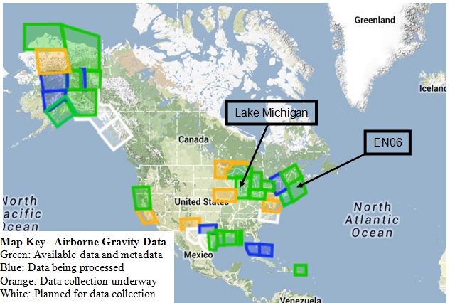
Figure 2 Extents of GRAV-D Collections as of 11 February 2014. Inset box in lower left gives legend on status of blocks. EN06 block in NE U.S.A. (Maine) and Lake Michigan are discussed further below.

The GRAV-D Project has completed 35% of the U.S. regions and is well on track for completion before 2022. Figure 2 highlights the status as of 11 February 2014. For up to date information, see http://www.ngs.noaa.gov/GRAV-D/data_products.shtml. A typical block is planned to be flown at 6.1 km (20,000 ft), with data lines spaced 10 km apart, and flown at about 220 knots (~407 km/h. GPS, IMU, and gravity meter readings are obtained and processed into a Level 1 product available for download from the GRAV-D website. A general description of how these products are developed is provided in the next section.

2.2 Data Collection and Processing

What is the waveband of reliability for the airborne gravity data? The upper limit is determined by the shortest dimensions of the survey block. Most GRAV-D surveys are rectangular and 400 km by 500 km in size to overlap the shortest wavebands of GRACE (300-400 km) and GOCE (100-200 km) satellite gravity data. The shortest wavelength in the airborne gravity is defined by sampling theory to be twice the sampling interval, which in the cross track direction is twice the data line spacing, or 20 km at full resolution or 10 km at half-resolution. Data resolution along track is somewhat shorter than this, and is determined by a combination of flight altitude (Childers et al 1999) and the amount of along-track low-pass filtering used. At 6.1 km altitude, gravity features below roughly 6 km in width (i.e. wavelengths below 12 km) are unlikely to be resolved. The along-track low pass filtering also reduces the resolution of the signal, as a function of aircraft velocity and filtering length. Data are measured at a 1 second rate which provides a measurement every 113 meters (at the nominal 220 knots velocity). A 120s time-domain Gaussian low pass filter is applied sequentially three times, and based upon the nominal speed of the aircraft, the filter is likely to suppress wavelengths below ~13 km. Thus there is more spectral information in the direction of the data lines (13 km minimum) than in the cross line direction (20 km minimum). Hence for data collected at 6.1 km altitude, the gravity data exist within the spectral band of 20 km to 400 km although the satellite data are deemed to be more reliable in the long (300-400 km) wavelengths. At 10 km altitude, the waveband signal is essentially the same as the 6.1 km data because it is determined by the data line spacing and the survey block dimensions, although the higher altitude attenuates signal amplitude and results in greater noise in the downward-continued product.

Further detailed information about the airborne gravity data collection and processing for all blocks is available online at the GRAV-D webpage along with the data at http://www.ngs.noaa.gov/GRAV-D/. Also available at the website is documentation for the aerogravity data collection process and a survey report for each survey block.

3. ANALYSIS

The NGS Geoid Team is the primary customer for the aerogravity data and is responsible for developing the required cm-level accurate geoid height model for 2022. Systematic errors are first removed or reduced in individual aerogravity profiles to better determine the geophysical signal present as a Level 2 product. Then the aerogravity may be used to assess the surface gravity data from the NGS database.

The next two subsections cover both these aspects. A simplified approach to bias removal in individual aerogravity profiles is provided over the Northeastern U.S. (Maine). Blocks EN06, EN07 and EN09 are used and also highlight the potential errors in the surface gravity data used in EGM2008. These were flown in 2012 and processed in 2013. To demonstrate how aerogravity can then be used to evaluate surface gravity data, the EN03 survey is used over Lake Michigan in the Great Lakes region where significant surface gravity data problems are known to exist. Block EN03 was collected and flown in 2013.

3.1 Northeastern U.S.A.

Figure 2 shows the location of a block of data (EN06) spanning coastal Maine. The nearby green blocks are EN07 and EN09. The intent of this subsection is to highlight how the aerogravity can be compared against a global gravity field model that already contains short wavelength signal derived from surface gravity data. The supposition here is that systematic errors from surface gravity data used in the global model contain biases and trends that will be detected by the aerogravity. These biases and trends will show up as systematic differences that will be highlighted in a plot of the differences between the aerogravity and the SHM containing the surface gravity data. An SHM was derived from the GOCO03S (Mayer-Gürr 2012) in combination with the terrestrial grid for EGM2008 (Pavlis et al. 2012). This improved reference model incorporates more GOCE signal while retaining the short wavelength signal from the surface gravity used to build EGM2008. Using this SHM, gravity disturbances were predicted at the aerogravity observation points to form residuals.

Both the SHM and the aerogravity contain signal between 20-400 km wavelengths. The aerogravity data were also tied to ground control when the aircraft was launched and landed. So ideally there should also be no long wavelength differences. Signal below 20 km would have little power and would be negligible. Hence these residuals should be near zero if the signal detected by the aerogravity were consistent with both the existing surface gravity data used in EGM2008 and that from the GOCO03S satellite data.

Figure 3a highlights the residuals in grid EN06. Note that many profiles show evidence of an unremoved bias or some systematic effect ("trackiness"). The averages these residual profiles were used to determine biases (Figure 3b), which were removed from the original residual profiles. This residual profiles with the means removed are shown for Blocks EN06, EN07, and EN09 (Figure 3c). Clear features are seen that correlate between tracks indicating that there are real geophysical signal differences between what is detected by the aerogravity and what is indicated by the surface gravity data inherent in EGM2008. The magnitude of these features is in the range of 3-5 mGals but they correlate across a hundred or more kilometers.

This is a near shore region and so a number of sources constitute the EGM2008 surface data. Data offshore were derived from satellite altimeters. This data tends to break down in the near shore environment and in backwater areas (Sandwell, 1990). Significant negative and positive features can be seen to extend along the shoreline and in bay areas in Figure 3.c. Onshore, data derived from terrestrial gravity surveys, which were corrected for elevation and other parameters. The SW-NE trending highs and lows correspond to features in the terrain, which could indicate problems with the gravity observations or the terrain models.

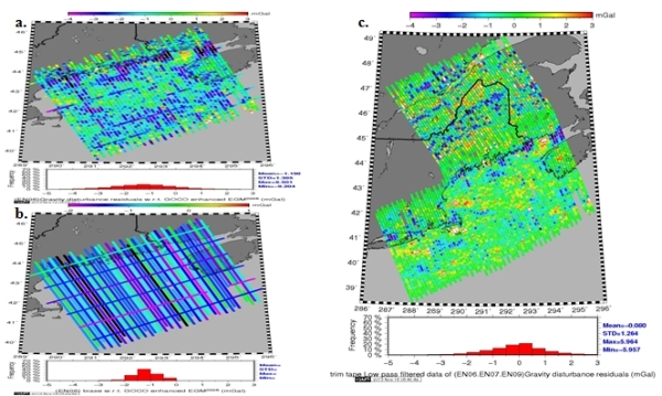
Figure 3 a. Residual gravity disturbances (EN06 – SHM). b. Biases detected in EN06 profiles. c. EN06, EN07, and EN09 residual gravity disturbances with biases removed. Remaining features highlight differences between aerogravity and surface gravity from the reference SHM. Residual features with lateral extents across multiple profiles indicate real signal not just noise.

Additionally, the boundaries between the three surveys are not strongly in evidence. Each of the surveys was planned with some overlap to ensure continuous coverage and processed using the same techniques. As a result, no systematic features exist between survey blocks, and the combined model of all three presents a consistent treatment of the residual gravity disturbances throughout the region (i.e., there are no biases between the survey blocks).

There are likely some problems with determining biases using this approach. If, as shown in Figure 3c., there are systematic differences between the aerogravity signal and the surface data, then this shorter wavelength signal slightly alters the overall average resulting in an incorrectly determined bias value. However, the above procedure removes these potential biases to a first order. Further refinements will be required to better remove biases of the aerogravity with respect to only the satellite signal at the longest wavelengths. However, the fact that the differences exist between the aerogravity and the existing surface data indicates that the aerogravity has discovered some potential systematic errors in the surface gravity that may preclude a cm-level accurate solution. Surface gravity surveys will next be compared against aerogravity to determine the magnitude of the biases in the terrestrial surveys.

3.2 Lake Michigan

It is desirable to see if any of the surface gravity data held by NGS contain biases or trends that would impact geoid modeling. In the previous subsection, it was shown that surface gravity commonly used in developing global SHM had systematic differences that may represent biases in that data. To develop a regional geoid of sufficient accuracy, it is desirable to detect any such errors in the NGS surface gravity data using the aerogravity. Satellite models will likely pick up these differences as well but will not sufficiently resolve the biases for individual surface gravity surveys.

Aerogravity data for block EN03 were treated in a similar manner as above. The next step in the process is to harmonically capture this signal using Least Squares Collocation (LSC) in order to make the data regular for capture into a SHM. Since the SHM is a global function, the aerogravity are used to update the local region of the block survey, while retaining the original signal outside of the region. The residual gravity highlights the difference between what the aerogravity sensed and what was indicated by the reference model at scales between 20-400 km. By modeling and incorporating these residuals into an updated SHM, the local gravity field will reflect what was sensed by the aerogravity and not was previously based on the surface gravity data in EGM2008. As the GRAV-D Project progresses, more blocks will be available to build into a larger region. In Figure 3 above, three blocks were assembled. There are more than five blocks available for the Great Lakes.

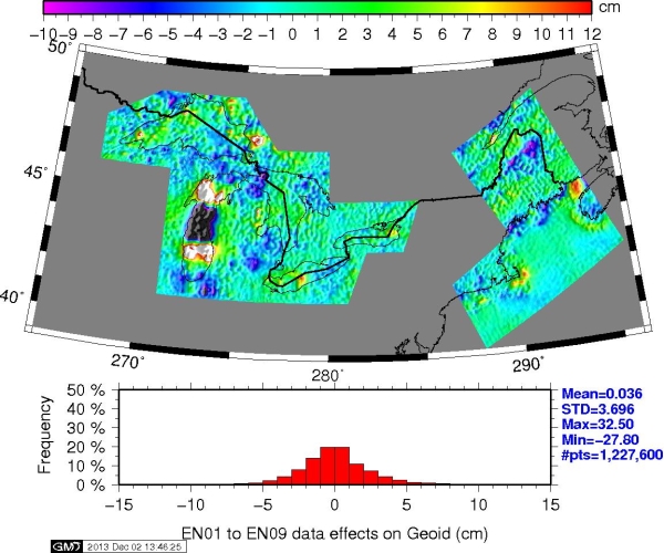
Figure 4 Equivalent residual geoid signal to that shown in Figure 3.c. Given for GRAV-D aerogravity blocks over the Northeast U.S. (EN06, EN07, EN09) and Great Lakes (EN01, EN02, EN03, EN04, EN05).

The process used to develop the residual gravity data shown in Figure 3c for the Northeast U.S. was repeated for the Great Lakes region. Figure 4, shows the equivalent residual geoid signal implied by the residual gravity data for the Northeast U.S. and the Great Lakes regions. Note that 3-5 mGal features seen in Figure 3c over Maine translate to 5-10 cm features in the geoid. Systematic differences in gravity over a hundred kilometers have decimeter impacts on derived geoid heights. Hence, incorporating the aerogravity would improve the regional geoid model by modifying surface gravity signal (short wavelengths) derived from SHM. However, it would be better to not rely on modifying the suspect surface gravity data after it was incorporated into a SHM. A better approach would be to remove any biases, trends, or other systematic effects from the surface gravity data before combining them into a regional geoid.

The next step after this would be to predict gravity values from this aerogravity modified SHM at the surface gravity point locations. However, when this process was developed over other regions in the Great Lakes, significant ringing occurred. This is normally an indication of applying too narrow a filter during Spherical Harmonic Analysis. At the time of this analysis, the issue has not been adequately resolved to enable a direct comparison using this approach. An alternative approach was devised that permitted comparison of the aerogravity signal to existing surface gravity data.

Figure 5 Difference between aerogravity and surface gravity held in the NGS database. Clear positive (above +10 mGals) biases are seen in track cluster (red boxes) that bound a cluster of tracks in the middle (magenta box) where pronounced negative (below -10 mGals) biases are seen. The scale of these biases would produce significant systematic errors in derived geoid height models.

The LSC-generated residual gravity grid was instead analytically downward continued to the surface. This effectively permits predictions of the residual values at the locations of surface gravity survey points. Since the surface gravity have full signal, the original (GOCO03S-EGM2008) SHM was removed from them to produce a second set of residuals gravity values. Both sets of residuals have been reduced by removing the same SHM. Hence, taking the difference of both sets of residuals highlights the differences between the aerogravity and the surface data (Figure 5).This double differencing effectively removes the SHM from the equation, because it is common to both.

Most data fall into an acceptable range of residual values. Certainly, they will all need to be addressed. However, several clusters of profiles are seen that have significant systematic effects (in red and magenta boxes). The cluster of profile lines in the middle of the Lake are off the bottom of the color scale (black) below -10 mGals in magnitude, while the clusters above and below that are off the top of the color scale (white) at +10 mGals. Moving from North to South over these features produces a sharp 20 mGal drop followed by a sharp 20 mGal rise. This feature is clearly seen over Lake Michigan in the same region in the residual geoid showing signal differences between the aerogravity and EGM2008 signal in Figure 4. Removal of these biases is essential if the surface gravity data are to be optimally combined with the satellite and airborne gravity data into a seamless gravity field model.

Figure 6 Differences between EGM2008 and GOCO03S through degree 120. Notte that the systematic feature seen in Figure 5 over central Lake Michigan are seen here but only broadly.

Figure 6 shows the difference between EGM2008 and GOCO03 filtered to degree 120. This effectively highlights the GOCE signal in the middle to long wavelengths of the gravity field. Of note, the same feature is seen over central Lake Michigan as was seen in Figure 4. Note the same broad structure with a high to the North and South of a central low. So GOCE would appear to have likewise determined this same systematic difference with EGM2008. However, the GOCE signal is too broad to be of use in detecting which specific surface gravity profiles need to be evaluated for potential biases such as was seen in Figure 5. While the GOCE-EGM2008 comparison could likely be made as high as degree 180, this would still be too coarse to enable evaluation of individual surface gravity profiles as in Figure 5.

4. OUTLOOK AND FUTURE WORK

The National Geodetic Survey will define new geometric and geophysical datums in 2022 to replace NAD 83 and NAVD 88 for the United States. This paper focused on the aerogravity collected as a part of the GRAV-D Project to be used for a geoid height model to serve as the realization of that future vertical datum. Canada has already adopted a similar datum and Mexico and many other countries in North and Central America are likewise interested in collaborating on common geoid models to serve as a regional height system.

Satellite data developed from missions such as GRACE and GOCE provide the long wavelength control that will unify height systems both at continental scales and as a part of a World height System. In turn, the aerogravity data are used to strengthen and enhance the middle wavelengths for the model over the U.S.A. Surface gravity data will provide the fine detail at the shortest wavelengths. The aim is to meld these data sets starting with the satellite data, then incorporating the aerogravity and finally then using the signal from surface gravity data - building progressively to a higher resolution model. The intent is to get away from reliance on existing SHM's developed using suspect surface gravity data. This will provide a seamless gravity field model in spectral content as well as spatial content, because the GRAV D Project will extend well offshore on each coast and into neighboring countries. At this stage, systematic differences of between 3-8 mGals still exist in the aerogravity and in the surface data

Aerogravity processing continues to be refined in an effort to reduce these effects. The intent is not to rely upon the satellite data to remove them, but refine the processing techniques such that that aerogravity agrees with the satellite data in that portion of the gravity power spectrum where they overlap (transition band). These updates will result in multiple versions of the data even for the same block. Expect that the data available on the GRAV-D webpage will be updated periodically.

Some of the surface gravity data profiles held by NGS have been demonstrated also to have systematic differences with the aerogravity. These are likely biases in the surface gravity data whose source cannot be adequately resolved due to missing metadata. Hence, no refinements of processing techniques can resolve these. Aerogravity will be used to detect and mitigate these biases on a survey-by-survey basis.

As the aerogravity processing steps are developed, procedures for collection and processing will also be refined. These are already available and serve as basis for contracting some of the collection work. As these procedures become optimized, they will be available for others to use to develop standards for collection to be consistent with global gravity modeling efforts.

Processes for evaluating the surface gravity data must likewise be developed and improved. Determining an optimal method for combining data that does not produce ringing either in or out of the region is essential. Optimally satellite, airborne and surface gravity must be consistent over their respective transition bands as given in Figure 1. The aim is to have a seamless gravity field reliant upon satellite data at the longest wavelengths transitioning through to aerogravity and finally to surface gravity for the most local control.

It should be noted that the requirement is to define a geoid model for use as a vertical datum. A more optimal solution would be to generate a SHM that blends all sources. This would require an exceptionally large model (degree 10800) to achieve the current resolution of regional geoid models. This approach would expedite transformations between various functionals of the gravity field (gravity anomalies, gravity disturbances, geoid heights, deflections of the vertical) as well as between height systems (orthometric, normal, dynamic). It will remain a goal for research to see if this can be achieved.

There must also be outside metrics to validate the accuracy of any geoid model derived from this data. The Geoid Slope Validation Study for 2011 (GSVS11) is documented in Smith et al. (2013b) and is intended for just this purpose. A new model is planned for later this year (GSVS14) in a more gravimetrically challenging area (higher elevations, larger gravity changes though with generally flat terrain). There will likely be a third GSVS located in the Rocky Mountains to provide validation in high, rugged terrain.

Additional validation data sets that will be used include tidal bench marks in combination with Mean Ocean Dynamic Topography models for validation in coastal regions, astrogeodetic observations across the region, and minimally constrained GPS on leveled bench mark (GPSBM) data. The last is a normal step in developing existing vertical control for NAD 83 and NAVD 88. A minimally constrained solution is necessary for quality control before a constrained solution is used to make the official datum values. Minimal constraints should produce a series of geoid heights representative of the local geoid. As of 2014, GRAV D is on track for collections and development of the geoid processing techniques for implementation of a new vertical datum in 2022.

REFERENCES

Childers VA, RE Bell, and JM Brozena (1999) Airborne Gravimetry: An Investigation of Filtering, Geophysics, 64 (1), 61-69.

Drinkwater MR, R Haagmans, D Muzi, A Popescu, R Floberghagen, M Kern, and M Fehringer (2007) Proceedings of 3rd International GOCE User Workshop, 6-8 November, 2006, Frascati, Italy, ESA SP-627.

Mayer-Gürr T, D Rieser, E. Hoeck, JM Brockman, W-D Schuh, I Krasbutter, J Kusche, A Maier, S Krauss, W Hausleitner, O Baur, A Jaeggi, U Meyer, L Prange, R Pail, T Fecher, and T Gruber. (2012) The new combined satellite only model GOCO03S. Paper S2-183, GGHS Meeting in Venice, Italy 9-12 OCT 2012.

NGS (2013) National Geodetic Survey Ten-Year Strategic Plan, http://www.ngs.noaa.gov/web/news/Ten_Year_Plan_2013-2023.pdf

Pail R, S Bruinsma, F Migliaccio, C Foerste, H Goiginger, W-D Schuh, E Höck, M Reguzzoni, JM Brockmann, O Abrikosov, M Veicherts, T Fecher, R Mayrhofer, I Krasbutter, F Sansò, CC Tscherning (2011) First GOCE gravity field models derived by three different approaches, J. Geodesy, 85 (11), 819-843, DOI: 10.1007/s00190-011-0467-x.

Pavlis, NK, SA Holmes, SC Kenyon, and JK Factor (2012) The development and evaluation of the Earth Gravitational Model 2008 (EGM2008), JGR, 117 (B4), Article Number: B04406, DOI: 10.1029/2011JB008916.

Roman DR (2007) The Impact of Littoral Aerogravity on Coastal Geoid Heights, paper 9009, XXIV General Assembly of the I.U.G.G. in Perugia, Italy 2-13 July 2007.

Roman DR, D Winester, J Saleh (2010) Surface gravity observations define gravity field change over 30 years, Abstract G41A-0789 presented at 2010 Fall Meeting, AGU, San Francisco, Calif., 13-17 Dec.

Sandwell DT (1990) Geophysical Applications of Satellite Altimetry, Reviews of Geophysics Supplement, 132-137.

Saleh J, X Li, YM Wang, DR Roman, DA Smith (2013) Error analysis of the NGS’ surface gravity database, J. Geodesy, 87: 203¬221.

Smith D (2007) The GRAV-D project: Gravity for the Redefinition of the American Vertical Datum. Available online at: http://www.ngs.noaa.gov/GRAV-D/pubs/GRAV-D_v2007_12_19.pdf

Smith DA, M Véronneau, DR Roman, J Huang, YM Wang, and MG Sideris (2013a) Towards the Unification of the Vertical Datum Over the North American Continent. Chapter 36 in: Z Altamimi and X Collilieux (eds.), Reference Frames for Applications in Geosciences, International Association of Geodesy Symposia 138, DOI 10./1007/978-3-642-32998-2_36 © Springer-Verlag Heidelberg 2013.

Smith DA, SA Holmes, X Li, S Guillaume, YM Wang, B Bürki, DR Roman, and TM Damiani (2013b) Confirming regional 1 cm differential geoid accuracy from airborne gravimetry: the Geoid Slope Validation Survey of 2011, J. Geodesy, 87 (10-12), 885-907.

Snay R and T Soler (2000) Modern Terrestrial Reference Systems, Part 2: The Evolution of NAD 83, Professional Surveyor, February.

BIOGRAPHICAL NOTES

Daniel Roman is serving as the Chief (acting), Spatial Reference Systems Division at the U.S. National Geodetic Survey, while continuing to serve as the GRAV-D P.I. and Geoid Team Lead for development of a geoid height model in 2022 that will replace NAVD 88.

Xiaopeng Li is an employee of Data System Technology, Inc. and is contracted to NGS. He assists with spherical/ellipsoidal harmonic modeling efforts as well as geoid modeling efforts for various official and scientific purposes.

ACKNOWLEDGMENTS

The authors wish to thank our colleagues Dr. Simon Holmes, Dr. Vicki Childers, and Dr. Theresa Damiani for their generous support in developing this paper.

CONTACTS

Dr. Daniel Roman
National Geodetic Survey
SSMC 3, N/NGS6, #8813
1315 East-West Highway
Silver Spring MD 20910
U.S.A.
Tel. +1-301-713-3200 x103
Fax + 1-301-713-4324
Email: dan.roman@noaa.gov
Web site: http://www.ngs.noaa.gov/GRAV-D/
http://www.ngs.noaa.gov/GEOID/